29. Job Search II: Search and Separation #

Contents

Job Search II: Search and Separation

29.1. Overview #

Previously we looked at the McCall job search model [McC70] as a way of understanding unemployment and worker decisions.

One unrealistic feature of the model is that every job is permanent.

In this lecture we extend the McCall model by introducing job separation.

Once separation enters the picture, the agent comes to view

the loss of a job as a capital loss, and
a spell of unemployment as an investment in searching for an acceptable job

using LinearAlgebra, Statistics
using Distributions, LaTeXStrings, NLsolve, Plots

29.2. The Model #

The model concerns the life of an infinitely lived worker and

the opportunities he or she (let’s say he to save one character) has to work at different wages
exogenous events that destroy his current job
his decision making process while unemployed

The worker can be in one of two states: employed or unemployed.

He wants to maximize

(29.1)#

E \sum_{t = 0}^{\infty} β^{t} u (Y_{t})

The only difference from the baseline model is that we’ve added some flexibility over preferences by introducing a utility function $u$ .

It satisfies $u^{'} > 0$ and $u^{″} < 0$ .

29.2.1. Timing and Decisions#

Here’s what happens at the start of a given period in our model with search and separation.

If currently employed, the worker consumes his wage $w$ , receiving utility $u (w)$ .

If currently unemployed, he

receives and consumes unemployment compensation $c$
receives an offer to start work next period at a wage $w^{'}$ drawn from a known distribution $p_{1}, \dots, p_{n}$

He can either accept or reject the offer.

If he accepts the offer, he enters next period employed with wage $w^{'}$ .

If he rejects the offer, he enters next period unemployed.

When employed, the agent faces a constant probability $α$ of becoming unemployed at the end of the period.

(Note: we do not allow for job search while employed—this topic is taken up in a later lecture)

29.3. Solving the Model using Dynamic Programming #

Let

$V (w)$ be the total lifetime value accruing to a worker who enters the current period employed with wage $w$ .
$U$ be the total lifetime value accruing to a worker who is unemployed this period.

Here value means the value of the objective function (29.1) when the worker makes optimal decisions at all future points in time.

Suppose for now that the worker can calculate the function $V$ and the constant $U$ and use them in his decision making.

Then $V$ and $U$ should satisfy

(29.2)#

V (w) = u (w) + β [(1 - α) V (w) + α U]

and

(29.3)#

U = u (c) + β \sum_{i} max {U, V (w_{i})} p_{i}

Let’s interpret these two equations in light of the fact that today’s tomorrow is tomorrow’s today.

The left hand sides of equations (29.2) and (29.3) are the values of a worker in a particular situation today.
The right hand sides of the equations are the discounted (by $β$ ) expected values of the possible situations that worker can be in tomorrow.
But tomorrow the worker can be in only one of the situations whose values today are on the left sides of our two equations.

Equation (29.3) incorporates the fact that a currently unemployed worker will maximize his own welfare.

In particular, if his next period wage offer is $w^{'}$ , he will choose to remain unemployed unless $U < V (w^{'})$ .

Equations (29.2) and (29.3) are the Bellman equations for this model.

Equations (29.2) and (29.3) provide enough information to solve out for both $V$ and $U$ .

Before discussing this, however, let’s make a small extension to the model.

29.3.1. Stochastic Offers#

Let’s suppose now that unemployed workers don’t always receive job offers.

Instead, let’s suppose that unemployed workers only receive an offer with probability $γ$ .

If our worker does receive an offer, the wage offer is drawn from $p$ as before.

He either accepts or rejects the offer.

Otherwise the model is the same.

With some thought, you will be able to convince yourself that $V$ and $U$ should now satisfy

(29.4)#

V (w) = u (w) + β [(1 - α) V (w) + α U]

and

(29.5)#

U = u (c) + β (1 - γ) U + β γ \sum_{i} max {U, V (w_{i})} p_{i}

29.3.2. Solving the Bellman Equations#

We’ll use the same iterative approach to solving the Bellman equations that we adopted in the first job search lecture.

Here this amounts to

make guesses for $U$ and $V$
plug these guesses into the right hand sides of (29.4) and (29.5)
update the left hand sides from this rule and then repeat

In other words, we are iterating using the rules

(29.6)#

V_{n + 1} (w_{i}) = u (w_{i}) + β [(1 - α) V_{n} (w_{i}) + α U_{n}]

and

(29.7)#

U_{n + 1} = u (c) + β (1 - γ) U_{n} + β γ \sum_{i} max {U_{n}, V_{n} (w_{i})} p_{i}

starting from some initial conditions $U_{0}, V_{0}$ .

Formally, we can define a “Bellman operator” T which maps:

(29.8)#

T V (\cdot) = u (\cdot) + β (1 - α) V (\cdot) + α U

In which case we are searching for a fixed point

(29.9)#

T V^{*} = V^{*}

As before, the system always converges to the true solutions—in this case, the $V$ and $U$ that solve (29.4) and (29.5).

A proof can be obtained via the Banach contraction mapping theorem.

29.4. Implementation #

Let’s implement this iterative process

using Distributions, LinearAlgebra, NLsolve, Plots

function solve_mccall_model(mcm; U_iv = 1.0, V_iv = ones(length(mcm.w)),
                            tol = 1e-5,
                            iter = 2_000)
    (; alpha, beta, sigma, c, gamma, w, dist, u, p) = mcm

    # parameter validation
    @assert c > 0.0
    @assert minimum(w) > 0.0 # perhaps not strictly necessary, but useful here

    # necessary objects
    u_w = mcm.u.(w, sigma)
    u_c = mcm.u(c, sigma)

    # Bellman operator T. Fixed point is x* s.t. T(x*) = x*
    function T(x)
        V = x[1:(end - 1)]
        U = x[end]
        [u_w + beta * ((1 - alpha) * V .+ alpha * U);
         u_c + beta * (1 - gamma) * U + beta * gamma * dot(max.(U, V), p)]
    end

    # value function iteration
    x_iv = [V_iv; U_iv] # initial x val
    xstar = fixedpoint(T, x_iv, iterations = iter, xtol = tol, m = 0).zero
    V = xstar[1:(end - 1)]
    U = xstar[end]

    # compute the reservation wage
    wbarindex = searchsortedfirst(V .- U, 0.0)
    if wbarindex >= length(w) # if this is true, you never want to accept
        w_bar = Inf
    else
        w_bar = w[wbarindex] # otherwise, return the number
    end

    # return a NamedTuple, so we can select values by name
    return (; V, U, w_bar)
end

solve_mccall_model (generic function with 1 method)

The approach is to iterate until successive iterates are closer together than some small tolerance level.

We then return the current iterate as an approximate solution.

Let’s plot the approximate solutions $U$ and $V$ to see what they look like.

We’ll use the default parameterizations found in the code above.

function mcall_model(; alpha = 0.2,
                     beta = 0.98, # discount rate
                     gamma = 0.7,
                     c = 6.0, # unemployment compensation
                     sigma = 2.0,
                     u = (c, sigma) -> (c^(1 - sigma) - 1) / (1 - sigma),
                     w = range(10, 20, length = 60), # wage values
                     dist = BetaBinomial(59, 600, 400)) # distribution over wage values
    p = pdf.(dist, support(dist))
    return (; alpha, beta, gamma, c, sigma, u, w, dist, p)
end

mcall_model (generic function with 1 method)

# plots setting

mcm = mcall_model()
(; V, U) = solve_mccall_model(mcm)
U_vec = fill(U, length(mcm.w))

plot(mcm.w, [V U_vec], lw = 2, alpha = 0.7, label = [L"V" L"U"])

The value $V$ is increasing because higher $w$ generates a higher wage flow conditional on staying employed.

At this point, it’s natural to ask how the model would respond if we perturbed the parameters.

These calculations, called comparative statics, are performed in the next section.

29.5. The Reservation Wage #

Once $V$ and $U$ are known, the agent can use them to make decisions in the face of a given wage offer.

If $V (w) > U$ , then working at wage $w$ is preferred to unemployment.

If $V (w) < U$ , then remaining unemployed will generate greater lifetime value.

Suppose in particular that $V$ crosses $U$ (as it does in the preceding figure).

Then, since $V$ is increasing, there is a unique smallest $w$ in the set of possible wages such that $V (w) \geq U$ .

We denote this wage $\bar{w}$ and call it the reservation wage.

Optimal behavior for the worker is characterized by $\bar{w}$

if the wage offer $w$ in hand is greater than or equal to $\bar{w}$ , then the worker accepts
if the wage offer $w$ in hand is less than $\bar{w}$ , then the worker rejects

If $V (w) < U$ for all $w$ , then the function returns np.inf.

Let’s use it to look at how the reservation wage varies with parameters.

In each instance below we’ll show you a figure and then ask you to reproduce it in the exercises.

29.5.1. The Reservation Wage and Unemployment Compensation#

First, let’s look at how $\bar{w}$ varies with unemployment compensation.

In the figure below, we use the default parameters in the mcall_model tuple, apart from c (which takes the values given on the horizontal axis)

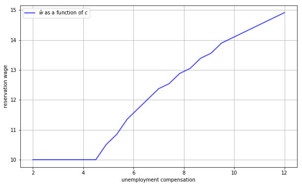
As expected, higher unemployment compensation causes the worker to hold out for higher wages.

In effect, the cost of continuing job search is reduced.

29.5.2. The Reservation Wage and Discounting#

Next let’s investigate how $\bar{w}$ varies with the discount rate.

The next figure plots the reservation wage associated with different values of $β$

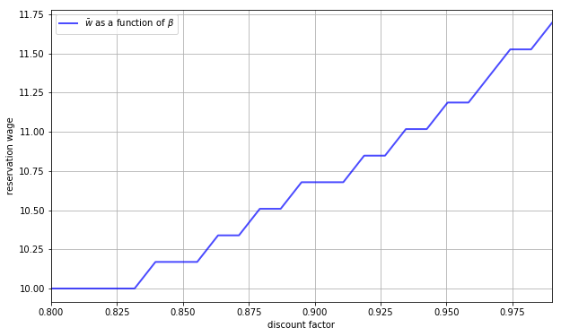
Again, the results are intuitive: More patient workers will hold out for higher wages.

29.5.3. The Reservation Wage and Job Destruction#

Finally, let’s look at how $\bar{w}$ varies with the job separation rate $α$ .

Higher $α$ translates to a greater chance that a worker will face termination in each period once employed.

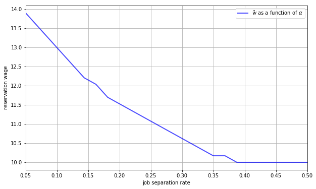
Once more, the results are in line with our intuition.

If the separation rate is high, then the benefit of holding out for a higher wage falls.

Hence the reservation wage is lower.

29.6. Exercises #

29.6.1. Exercise 1#

Reproduce all the reservation wage figures shown above.

29.6.2. Exercise 2#

Plot the reservation wage against the job offer rate $γ$ .

Use

gamma_vals = range(0.05, 0.95, length = 25)

0.05:0.0375:0.95

Interpret your results.

29.7. Solutions #

29.7.1. Exercise 1#

Using the solve_mccall_model function mentioned earlier in the lecture, we can create an array for reservation wages for different values of $c$ , $β$ and $α$ and plot the results like so

c_vals = range(2, 12, length = 25)

models = [mcall_model(c = cval) for cval in c_vals]
sols = solve_mccall_model.(models)
w_bar_vals = [sol.w_bar for sol in sols]

plot(c_vals,
     w_bar_vals,
     lw = 2,
     alpha = 0.7,
     xlabel = "unemployment compensation",
     ylabel = "reservation wage",
     label = L"$\overline{w}$ as a function of $c$")

Note that we could’ve done the above in one pass (which would be important if, for example, the parameter space was quite large).

w_bar_vals = [solve_mccall_model(mcall_model(c = cval)).w_bar
              for cval in c_vals];
# doesn't allocate new arrays for models and solutions

29.7.2. Exercise 2#

Similar to above, we can plot $\bar{w}$ against $γ$ as follows

gamma_vals = range(0.05, 0.95, length = 25)

models = [mcall_model(gamma = gammaval) for gammaval in gamma_vals]
sols = solve_mccall_model.(models)
w_bar_vals = [sol.w_bar for sol in sols]

plot(gamma_vals, w_bar_vals, lw = 2, alpha = 0.7, xlabel = "job offer rate",
     ylabel = "reservation wage",
     label = L"$\overline{w}$ as a function of $\gamma$")

As expected, the reservation wage increases in $γ$ .

This is because higher $γ$ translates to a more favorable job search environment.

Hence workers are less willing to accept lower offers.