30. A Problem that Stumped Milton Friedman#

30.1. Overview#

This lecture describes a statistical decision problem encountered by Milton Friedman and W. Allen Wallis during World War II when they were analysts at the U.S. Government’s Statistical Research Group at Columbia University.

This problem led Abraham Wald [Wal47] to formulate sequential analysis, an approach to statistical decision problems intimately related to dynamic programming.

In this lecture, we apply dynamic programming algorithms to Friedman and Wallis and Wald’s problem.

Key ideas in play will be:

• Bayes’ Law

• Dynamic programming

• Type I and type II statistical errors

  • a type I error occurs when you reject a null hypothesis that is true

  • a type II error is when you accept a null hypothesis that is false

• Abraham Wald’s sequential probability ratio test

• The power of a statistical test

• The critical region of a statistical test

• A uniformly most powerful test

30.2. Origin of the problem#

On pages 137-139 of his 1998 book Two Lucky People with Rose Friedman [FF98], Milton Friedman described a problem presented to him and Allen Wallis during World War II, when they worked at the US Government’s Statistical Research Group at Columbia University.

Let’s listen to Milton Friedman tell us what happened.

“In order to understand the story, it is necessary to have an idea of a simple statistical problem, and of the standard procedure for dealing with it. The actual problem out of which sequential analysis grew will serve. The Navy has two alternative designs (say A and B) for a projectile. It wants to determine which is superior. To do so it undertakes a series of paired firings. On each round it assigns the value 1 or 0 to A accordingly as its performance is superior or inferior to that of B and conversely 0 or 1 to B. The Navy asks the statistician how to conduct the test and how to analyze the results.

“The standard statistical answer was to specify a number of firings (say 1,000) and a pair of percentages (e.g., 53% and 47%) and tell the client that if A receives a 1 in more than 53% of the firings, it can be regarded as superior; if it receives a 1 in fewer than 47%, B can be regarded as superior; if the percentage is between 47% and 53%, neither can be so regarded.

“When Allen Wallis was discussing such a problem with (Navy) Captain Garret L. Schyler, the captain objected that such a test, to quote from Allen’s account, may prove wasteful. If a wise and seasoned ordnance officer like Schyler were on the premises, he would see after the first few thousand or even few hundred [rounds] that the experiment need not be completed either because the new method is obviously inferior or because it is obviously superior beyond what was hoped for $\dots$ ‘’

Friedman and Wallis struggled with the problem but, after realizing that they were not able to solve it, described the problem to Abraham Wald.

That started Wald on the path that led him to Sequential Analysis [Wal47].

We’ll formulate the problem using dynamic programming.

30.3. A dynamic programming approach#

The following presentation of the problem closely follows Dmitri Berskekas’s treatment in Dynamic Programming and Stochastic Control [Ber75].

A decision maker observes iid draws of a random variable $z$.

He (or she) wants to know which of two probability distributions $f_0$ or $f_1$ governs $z$.

After a number of draws, also to be determined, he makes a decision as to which of the distributions is generating the draws he observers.

To help formalize the problem, let $x\in \{x_0,x_1\}$ be a hidden state that indexes the two distributions:

Before observing any outcomes, the decision maker believes that the probability that $x=x_0$ is

After observing $k+1$ observations $z_k,z_{k-1},\dots ,z_0$, he updates this value to

which is calculated recursively by applying Bayes’ law:

After observing $z_k,z_{k-1},\dots ,z_0$, the decision maker believes that $z_{k+1}$ has probability distribution

This is a mixture of distributions $f_0$ and $f_1$, with the weight on $f_0$ being the posterior probability that $x=x_0$ 1.

To help illustrate this kind of distribution, let’s inspect some mixtures of beta distributions.

The density of a beta probability distribution with parameters $a$ and $b$ is

We’ll discretize this distribution to make it more straightforward to work with.

The next figure shows two discretized beta distributions in the top panel.

The bottom panel presents mixtures of these distributions, with various mixing probabilities $p_k$.

using LinearAlgebra, Statistics, Interpolations, NLsolve
using Distributions, LaTeXStrings, Random, Plots, FastGaussQuadrature, SpecialFunctions, StatsPlots

base_dist = [Beta(1, 1), Beta(3, 3)]
mixed_dist = MixtureModel.(Ref(base_dist),
                           (p -> [p, one(p) - p]).(0.25:0.25:0.75))
plot(plot(base_dist, labels = [L"f_0" L"f_1"],
          title = "Original Distributions"),
     plot(mixed_dist, labels = [L"1/4-3/4" L"1/2-1/2" L"3/4-1/4"],
          title = "Distribution Mixtures"),
     # Global settings across both plots
     ylab = "Density", ylim = (0, 2), layout = (2, 1))

30.3.3. Intuition#

Let’s try to guess what an optimal decision rule might look like before we go further.

Suppose at some given point in time that $p$ is close to 1.

Then our prior beliefs and the evidence so far point strongly to $x=x_0$.

If, on the other hand, $p$ is close to 0, then $x=x_1$ is strongly favored.

Finally, if $p$ is in the middle of the interval $[0,1]$, then we have little information in either direction.

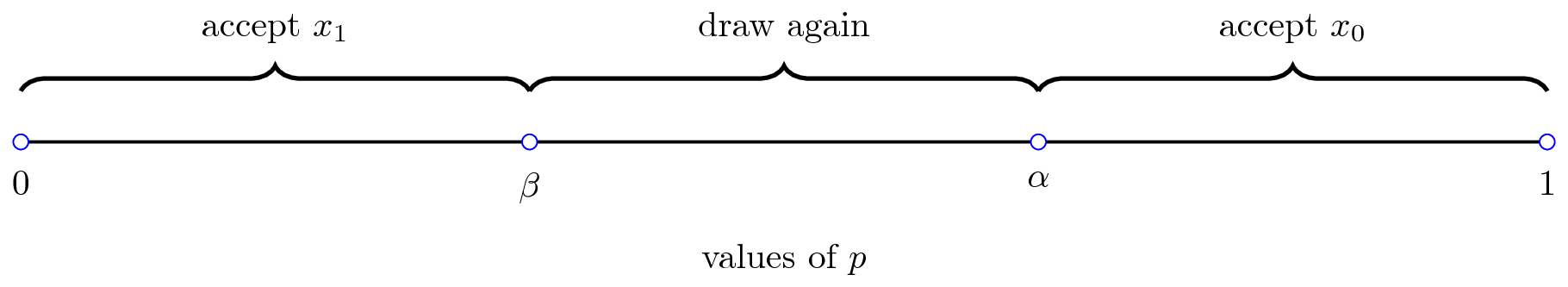
This reasoning suggests a decision rule such as the one shown in the figure

As we’ll see, this is indeed the correct form of the decision rule.

The key problem is to determine the threshold values $\alpha ,\beta$, which will depend on the parameters listed above.

You might like to pause at this point and try to predict the impact of a parameter such as $c$ or $L_0$ on $\alpha$ or $\beta$.

30.4. Implementation#

Let’s code this problem up and solve it.

We discretize the belief space, set up quadrature rules for both likelihood distributions, and evaluate the Bellman operator on that grid. The helpers below encode the immediate losses, Bayes’ rule for the posterior belief, and the expectation of the continuation value in (30.4).

accept_x0(p, L0) = (one(p) - p) * L0
accept_x1(p, L1) = p * L1
const BELIEF_FLOOR = 1e-6

clamp_belief(p) = clamp(float(p), BELIEF_FLOOR, one(Float64) - BELIEF_FLOOR)

function gauss_jacobi_dist(F::Beta, N)
    s, wj = FastGaussQuadrature.gaussjacobi(N, F.β - 1, F.α - 1)
    x = (s .+ 1) ./ 2
    C = 2.0^(-(F.α + F.β - 1.0)) / SpecialFunctions.beta(F.α, F.β)
    return x, C .* wj
end

function wf_problem(; d0 = Beta(1, 1), d1 = Beta(9, 9), L0 = 2.0, L1 = 2.0,
                    c = 0.2, grid_size = 201, quad_order = 31)
    belief_grid = collect(range(BELIEF_FLOOR, one(Float64) - BELIEF_FLOOR,
                                length = grid_size))
    nodes0, weights0 = gauss_jacobi_dist(d0, quad_order)
    nodes1, weights1 = gauss_jacobi_dist(d1, quad_order)
    return (; d0, d1, L0 = float(L0), L1 = float(L1), c = float(c), belief_grid,
            nodes0, weights0, nodes1, weights1)
end

function posterior_belief(problem, p, z)
    (; d0, d1) = problem
    num = p * pdf(d0, z)
    den = num + (one(p) - p) * pdf(d1, z)
    return den == 0 ? clamp_belief(p) : clamp_belief(num / den)
end

function continuation_value(problem, p, vf)
    (; c, nodes0, weights0, nodes1, weights1) = problem

    loss(nodes,
         weights) = dot(weights, vf.(posterior_belief.(Ref(problem), p, nodes)))

    return c + p * loss(nodes0, weights0) +
           (one(p) - p) * loss(nodes1, weights1)
end

continuation_value (generic function with 1 method)

Next we solve a problem by applying value iteration to compute the value function and the associated decision rule.

function T(problem, v)
    (; belief_grid, L0, L1) = problem
    vf = LinearInterpolation(belief_grid, v, extrapolation_bc = Flat())
    out = similar(v)

    for (i, p) in enumerate(belief_grid)
        cont = continuation_value(problem, p, vf)
        out[i] = min(accept_x0(p, L0), accept_x1(p, L1), cont)
    end
    return out
end

function value_iteration(problem; tol = 1e-6, max_iter = 400)
    (; belief_grid, L0, L1) = problem
    v0 = [min(accept_x0(p, L0), accept_x1(p, L1)) for p in belief_grid]
    result = fixedpoint(v -> T(problem, v), v0)
    return result.zero
end

function decision_rule(problem; tol = 1e-6, max_iter = 400, verbose = false)
    values = value_iteration(problem; tol = tol, max_iter = max_iter)
    (; belief_grid, L0, L1) = problem
    vf = LinearInterpolation(belief_grid, values, extrapolation_bc = Flat())
    actions = similar(belief_grid, Int)

    for (i, p) in enumerate(belief_grid)
        stop0 = accept_x0(p, L0)
        stop1 = accept_x1(p, L1)
        cont = continuation_value(problem, p, vf)
        val = min(stop0, stop1, cont)
        actions[i] = isapprox(val, stop0; atol = 1e-5, rtol = 0) ? 1 :
                     isapprox(val, stop1; atol = 1e-5, rtol = 0) ? 2 : 3
    end

    beta_idx = findlast(actions .== 2)
    alpha_idx = findfirst(actions .== 1)
    beta = isnothing(beta_idx) ? belief_grid[1] : belief_grid[beta_idx]
    alpha = isnothing(alpha_idx) ? belief_grid[end] : belief_grid[alpha_idx]

    if verbose
        println("Accept x1 if p <= $(round(beta, digits=3))")
        println("Continue to draw if $(round(beta, digits=3)) <= p <= $(round(alpha, digits=3))")
        println("Accept x0 if p >= $(round(alpha, digits=3))")
    end

    return (; problem, alpha, beta, values, actions, vf)
end

function choice(p, rule)
    p = clamp_belief(p)
    stop0 = accept_x0(p, rule.problem.L0)
    stop1 = accept_x1(p, rule.problem.L1)
    cont = continuation_value(rule.problem, p, rule.vf)
    vals = (stop0, stop1, cont)
    idx = argmin(vals)
    return idx, vals[idx]
end

function simulator(problem; n = 100, p0 = 0.5, rng_seed = 0x12345678,
                   summarize = true, return_output = false, rule = nothing)
    rule = isnothing(rule) ? decision_rule(problem) : rule
    (; d0, d1, L0, L1, c) = rule.problem

    rng = MersenneTwister(rng_seed)
    outcomes = falses(n)
    costs = zeros(Float64, n)
    trials = zeros(Int, n)

    p_prior = clamp_belief(p0)

    for trial in 1:n
        p_current = p_prior
        truth = rand(rng, 1:2)
        dist = truth == 1 ? d0 : d1
        loss_if_wrong = truth == 1 ? L1 : L0
        draws = 0
        decision = 0

        while decision == 0
            draws += 1
            observation = rand(rng, dist)
            p_current = posterior_belief(rule.problem, p_current, observation)

            if p_current <= rule.beta
                decision = 2             # choose x1
            elseif p_current >= rule.alpha
                decision = 1             # choose x0
            end
        end

        correct = decision == truth
        outcomes[trial] = correct
        costs[trial] = draws * c + (correct ? 0.0 : loss_if_wrong)
        trials[trial] = draws
    end

    if summarize
        println("Correct: $(round(mean(outcomes), digits=2)), ",
                "Average Cost: $(round(mean(costs), digits=2)), ",
                "Average number of trials: $(round(mean(trials), digits=2))")
    end

    return return_output ? (rule.alpha, rule.beta, outcomes, costs, trials) :
           nothing
end

simulator (generic function with 1 method)

Random.seed!(0);
simulator(wf_problem());

Correct: 0.91, Average Cost: 0.54, 

Average number of trials: 1.81

Random.seed!(0);
simulator(wf_problem(; c = 0.4));

Correct: 0.79, Average Cost: 0.86, Average number of trials: 1.09

30.5. Comparison with Neyman-Pearson formulation#

For several reasons, it is useful to describe the theory underlying the test that Navy Captain G. S. Schuyler had been told to use and that led him to approach Milton Friedman and Allan Wallis to convey his conjecture that superior practical procedures existed.

Evidently, the Navy had told Captail Schuyler to use what it knew to be a state-of-the-art Neyman-Pearson test.

We’ll rely on Abraham Wald’s [Wal47] elegant summary of Neyman-Pearson theory.

For our purposes, watch for there features of the setup:

• the assumption of a fixed sample size $n$

• the application of laws of large numbers, conditioned on alternative probability models, to interpret the probabilities $\alpha$ and $\beta$ defined in the Neyman-Pearson theory

Recall that in the sequential analytic formulation above, that

• The sample size $n$ is not fixed but rather an object to be chosen; technically $n$ is a random variable.

• The parameters $\beta$ and $\alpha$ characterize cut-off rules used to determine $n$ as a random variable.

• Laws of large numbers make no appearances in the sequential construction.

In chapter 1 of Sequential Analysis [Wal47] Abraham Wald summarizes the Neyman-Pearson approach to hypothesis testing.

Wald frames the problem as making a decision about a probability distribution that is partially known.

(You have to assume that something is already known in order to state a well posed problem. Usually, something means a lot.)

By limiting what is unknown, Wald uses the following simple structure to illustrate the main ideas.

• A decision maker wants to decide which of two distributions $f_0$, $f_1$ govern an i.i.d. random variable $z$.

• The null hypothesis $H_0$ is the statement that $f_0$ governs the data.

• The alternative hypothesis $H_1$ is the statement that $f_1$ governs the data.

• The problem is to devise and analyze a test of hypothesis $H_0$ against the alternative hypothesis $H_1$ on the basis of a sample of a fixed number $n$ independent observations $z_1,z_2,\dots ,z_n$ of the random variable $z$.

To quote Abraham Wald,

• A test procedure leading to the acceptance or rejection of the hypothesis in question is simply a rule specifying, for each possible sample of size $n$, whether the hypothesis should be accepted or rejected on the basis of the sample. This may also be expressed as follows: A test procedure is simply a subdivision of the totality of all possible samples of size $n$ into two mutually exclusive parts, say part 1 and part 2, together with the application of the rule that the hypothesis be accepted if the observed sample is contained in part 2. Part 1 is also called the critical region. Since part 2 is the totality of all samples of size 2 which are not included in part 1, part 2 is uniquely determined by part 1. Thus, choosing a test procedure is equivalent to determining a critical region.

Let’s listen to Wald longer:

• As a basis for choosing among critical regions the following considerations have been advanced by Neyman and Pearson: In accepting or rejecting $H_0$ we may commit errors of two kinds. We commit an error of the first kind if we reject $H_0$ when it is true; we commit an error of the second kind if we accept $H_0$ when $H_1$ is true. After a particular critical region $W$ has been chosen, the probability of committing an error of the first kind, as well as the probability of committing an error of the second kind is uniquely determined. The probability of committing an error of the first kind is equal to the probability, determined by the assumption that $H_0$ is true, that the observed sample will be included in the critical region $W$. The probability of committing an error of the second kind is equal to the probability, determined on the assumption that $H_1$ is true, that the probability will fall outside the critical region $W$. For any given critical region $W$ we shall denote the probability of an error of the first kind by $\alpha$ and the probability of an error of the second kind by $\beta$.

Let’s listen carefully to how Wald applies a law of large numbers to interpret $\alpha$ and $\beta$:

• The probabilities $\alpha$ and $\beta$ have the following important practical interpretation: Suppose that we draw a large number of samples of size $n$. Let $M$ be the number of such samples drawn. Suppose that for each of these $M$ samples we reject $H_0$ if the sample is included in $W$ and accept $H_0$ if the sample lies outside $W$. In this way we make $M$ statements of rejection or acceptance. Some of these statements will in general be wrong. If $H_0$ is true and if $M$ is large, the probability is nearly $1$ (i.e., it is practically certain) that the proportion of wrong statements (i.e., the number of wrong statements divided by $M$) will be approximately $\alpha$. If $H_1$ is true, the probability is nearly $1$ that the proportion of wrong statements will be approximately $\beta$. Thus, we can say that in the long run [ here Wald applies a law of large numbers by driving $M\to \mathrm{\infty }$ (our comment, not Wald’s) ] the proportion of wrong statements will be $\alpha$ if $H_0$is true and $\beta$ if $H_1$ is true.

The quantity $\alpha$ is called the size of the critical region, and the quantity $1-\beta$ is called the power of the critical region.

Wald notes that

• one critical region $W$ is more desirable than another if it has smaller values of $\alpha$ and $\beta$. Although either $\alpha$ or $\beta$ can be made arbitrarily small by a proper choice of the critical region $W$, it is possible to make both $\alpha$ and $\beta$ arbitrarily small for a fixed value of $n$, i.e., a fixed sample size.

Wald summarizes Neyman and Pearson’s setup as follows:

• Neyman and Pearson show that a region consisting of all samples $(z_1,z_2,\dots ,z_n)$ which satisfy the inequality

  $$\frac{f_1(z_1)\cdots f_1(z_n)}{f_0(z_1)\cdots f_1(z_n)}\ge k$$

  is a most powerful critical region for testing the hypothesis $H_0$ against the alternative hypothesis $H_1$. The term $k$ on the right side is a constant chosen so that the region will have the required size $\alpha$.

Wald goes on to discuss Neyman and Pearson’s concept of uniformly most powerful test.

Here is how Wald introduces the notion of a sequential test

• A rule is given for making one of the following three decisions at any stage of the experiment (at the m th trial for each integral value of m ): (1) to accept the hypothesis H , (2) to reject the hypothesis H , (3) to continue the experiment by making an additional observation. Thus, such a test procedure is carried out sequentially. On the basis of the first observation one of the aforementioned decisions is made. If the first or second decision is made, the process is terminated. If the third decision is made, a second trial is performed. Again, on the basis of the first two observations one of the three decisions is made. If the third decision is made, a third trial is performed, and so on. The process is continued until either the first or the second decisions is made. The number n of observations required by such a test procedure is a random variable, since the value of n depends on the outcome of the observations.

1

Because the decision maker believes that $z_{k+1}$ is drawn from a mixture of two i.i.d. distributions, he does not believe that the sequence $[z_{k+1},z_{k+2},\dots ]$ is i.i.d. Instead, he believes that it is exchangeable. See [Kre88] chapter 11, for a discussion of exchangeability.